A blog to help electrical engineers and students to learn electrical engineering topics. Basic Electrical Engineering, Power Systems, Electrical Machines, tec.. Now special course on MATLAB for Beginners.

Class

Class

Monday, December 26, 2016

User Defined Functions in MATLAB Part -2


Previous post we discussed what is a user defined function in MATLAB. This lecture we will discuss how to define a function and how to call the function in a script.


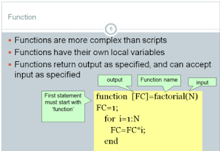
Components of a function is discussed in the previous lecture. The first statement in a function must be function definition.The basic syntax of a function definition is:

function[a, b, c]= basicmath(x,y)

Basically a function accepts an input vector, perform the operation, and returns a result. The sample function given has two input variables and three output variables. But we can also have functions without input or/and output.

Under some special occasions we may need some functions without any input or output.

Some functions will take some input arguments but will not return any output arguments. Functions to plot some shapes or curves and functions to display some message are examples.

A function can be called from the command window or inside a script or function. To run a function in command window, just type the name of comment with proper input and output arguments.


Thursday, December 1, 2016

User Defined Functions in MATLAB - Part 1


User-defined functions are similar to the MATLAB predefined functions. A function is a MATLAB program that can accept inputs and produce outputs. A function can be called or executed by another program or function. Code for a function is done in an Editor window or any text editor same way as script and saved as m-file. The m-file must have the same name as the function.

It is important that you give meaningful variable names to variables inside a function that you write, so that you and others can understand what the function does. The function M-file must be saved in your current directory.


The declaration statement 'function' is used to define the file as a function. It must be typed in lower case letters. Rules for giving function name is same as the rules for variable names.
Input arguments are typed in side the parentheses ( ). They are used to transfer data into function from calling program. Can be zero or more input arguments. 
Output arguments are typed inside the square brackets [ ]. They are used to transfer data out of function to calling program. Can be zero or more output arguments. It is important to give a meaningful variable names.

Tuesday, November 22, 2016

MATLAB Programming - Loop Control Part 2


In this lecture we will discuss more about Loop control.

- Switch – case commands

- Nested lops

- break command

- continue command

switch - case Command

There is no conditional statement used in this looping structure. It choose the code to be executed based on value of scalar or string, not just true/false. Different codes can be executed based on the value of the scalar defined in the switch command. The codes are defined using the case command.

Nested Loop

A nested loop is a loop or conditional statement placed inside another loop or conditional statement. Simply, a loop within a loop. Both for and while loops can be nested.

break Statement

The break statement terminates execution of for or while loop. Statements in the loop that appear after the break statement are not executed. In nested loops, break exits only from the loop in which it occurs. Control passes to the statement following the end of that loop.


continue Statement


The continue statement is used for passing control to next iteration of for or while loop. The continue statement in MATLAB works somewhat like the break statement. Instead of forcing termination, however, 'continue' forces the next iteration of the loop to take place, skipping any code in between.


Wednesday, October 26, 2016

MATLAB Script - Loop Control Part 1


In this lecture we will discuss about another flow control method – Loop control. A loop control is used to execute a set of commands repeatedly The set of commands is called the body of the loop.

MATLAB has two loop control techniques 
  1. Counted loops - executes commands a specified number of times. 
  2. Conditional loops - executes commands as long as a specified expression is true.
The counted loops are called ‘for’ loop and the conditional loops are called ‘while’ loop. The keyword “end” is used to show the end of a Loop.


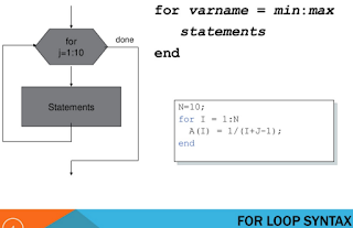
For loop is used when the numer of iteration is known. FOR Repeats for specified number of times ALWAYS executes computation loop at least once. For loop creates a vector of the variable defined in the command and execute the body of the loop for all the values of the vector. 

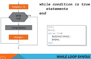
The while- loop used when the number of loop iterations is unknown. Number of iteration is controlled by a condition. The condition is tested in each iteration and stop looping when it is false. While loop will execute the body of loop ONLY if while condition is met. 

Both Scripts and functions also allow to loop using for and while loops. 

Conditional Control in MATLAB Scripts with Examples


In this lecture we discuss more about programming in MATLAB. One main section in programming is flow control. There are many flow control commands in MATLAB. In this lecture we discuss the conditional flow control commands.
Conditional statements are commands that allows MATLAB to decide whether or not to execute some code that follows the statement

Conditional statements use relational operators like ==,~=,>,< (Note that are all scalar tests).

The basic syntax is


žIf the conditional expression is true, MATLAB runs the lines of code that are between the line with if and the line with end.
If the conditional expression is false, MATLAB skips the code between if and the line with else and runs the code up to end.


Wednesday, September 21, 2016

MATLAB Scripts - Examples with Electrical Engineering Applications


This lecture we will practice some Basic MATLAB Scripts.
›We will start with simple scripts and will discuss some electrical engineering applications.

Program to calculate Electricity bill.

w = input('Enter power of your device (in watts): ');
h = input('Enter time (in hours): ');
r = input('Enter electricity rate (in dollars per KWH): ');
ec = w * h/1000 * r;
disp(’Your Electricity bill is’)
Disp(ec)


Power transfer vs Load resistance curve


RL = 1:0.01:10;
Vs = 12;
Rs = 2.5;
P = (Vs^2*RL)./(RL+Rs).^2;
plot(RL,P)
xlabel('Load resistance')
ylabel('Power dissipated')


Torque-Speed Curve for a squirrel cage Induction Motor 

›Ns=1500; % Synchronous speed;
›R1=15.6 ;R2=14;X1=18; X2=23;Xm=260;Vt=400/sqrt(3);
›s = 0.002:0.002:1; % vector of slip
›N = Ns.*(1-s); % Speed, in RPM
›Ws = 2*pi*Ns/60; % Synchronous speed in rad/sec
›Rr = R2./ s; % Rotor resistance
›Zr = j*X2 + Rr; % Total rotor impedance
›Za = j*Xm*Zr./(j*Xm+Zr); % Air-gap impedance
›Zt = R1 + j*X1 +Za; % Terminal impedance
›Ia = Vt ./ Zt; % Terminal Current
›I2 = j*Xm*Ia./(j*Xm+Zr); % Rotor Current
›Pag = 3* (abs(I2)).^2.*Rr; % Air-Gap Power
›Pm = Pag.* (1-s); % Converted Power
›Trq = Pag/ Ws; % Developed Torque
›subplot(2,1,1)
›plot(N, Trq)
›xlabel('Speed in RPM')
›ylabel('Torque (Nm)')
›subplot(2,1,2)
›plot(Ia, Trq)
›xlabel('Load Current')
›ylabel('Torque (Nm)')


Saturday, September 10, 2016

Introduction to MATLAB Scripts


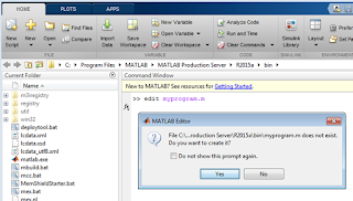
MATLAB Script or programs are sequences of MATLAB commands saved in plain text files. When you type the name of the script file at the MATLAB prompt the commands in the script file are executed as if you had typed them in command window. Code for a script is done in an Editor window and saved as m-file. 


In case your code has errors, MATLAB will show an error message in the command window, when you try to run the program . Error message will be hyperlinked to the line in the file that caused the error.

Script variables are added to the workspace. —If you use the same variables in another script, they will be modified by that script. —This may result in a confusing mix of variables in the MATLAB workspace. —Some times it may lead to a syntax error or may lead to subtle errors in the result.

Sunday, September 4, 2016

MATLAB Programming Tips 2 - Input and Output Commands


In this lecture we will review some common input and output commands in MATLAB. These commands are discussed in detail in previous lectures.
For detailed Lectures on Input and Output commands follow the links below.


Sunday, August 28, 2016

MATLAB Programming Tips Part 1


MATLAB program (functions and scripts) are stored as script file(.m files). This type of file contains MATLAB commands, so running it is equivalent to typing all the commands—one at a time—at the Command window prompt. You can run the file by typing its name at the Command window.


Matlab Programming Tips Part 1 from Shameer Ahmed Koya
  • Both functions and scripts are stored in .m files
  • —Type up a bunch of commands and save as filename.m
  • —Type filename in command window to run
  • Example: first_program.m
  • —The name of a script file must begin with a letter, and may include digits and the underscore character, up to 63 characters.
  • —Do not give a script file the same name as a variable.
  • —Do not give a script file the same name as a MATLAB command or function.

Tuesday, August 23, 2016

Polynomials and Curve Fitting in MATLAB


MATLAB provides a number of functions for the manipulation of polynomials. Polynomials are defined in MATLAB as row vectors made up of the coefficients of the polynomial, whose dimension is n+1, n being the degree of the polynomial. Polynomials in MATLAB vector must include all polynomial coefficients, even those that are zero.

MATLAB provides the function polyval to evaluate polynomials. MATLAB does not provide a direct function for adding or subtracting polynomials unless they are of the same order, when they are of the same order, normal matrix addition and subtraction applies. Polynomial multiplication is supported by the conv function. Where we want to divide one polynomial by another, in MATLAB we use the deconv function.

Polynomials and Curve Fitting in MATLAB from Shameer Ahmed Koya

Curve fitting is the process of adjusting a mathematical function so that it lays as closely as possible to a set of data points. MATLAB provides a number of ways to fit a curve to a set of measured data. One of these methods uses the “least squares” curve fit. This technique minimizes the squared errors between the curve and the set of measured data. The function polyfit solves the least squares polynomial curve fitting problem.

Friday, August 5, 2016

Working with Excel files in MATLAB - Part 2


Read part 1 here. We will discuss few more functions to deal with Excel files.

xlswrite ( ) – Write to Microsoft Excel spreadsheet file

xlswrite is a simple function to write data to an excel worksheet. The syntax is similar to the xlsread function
xlswrtie(‘filename’, A, ‘worksheet’, ‘range’)
The function write the values in the array A to the specified range of cells in the specified worksheet of the excel file. The array may be a numeric array, character array or a cell array depending on the data. The worksheet and range arguments are optional. If not specified, the data will be written to the first worksheet starting from A1.

Example:
No we will add marks of two more students to our grade file.
>> newstud = {342001, 'James', 12.5, 13, 20;342001, 'Anna', 12, 10.5, 16};


>> xlswrite('test.xlsx', newstud, 'A7:E8')

writetable( ) - Write table to file

wrtietable function by default write the content of martlab table to a text file in comma separated format. The file name will be automatically set if not specified.
writetable(T) is the basic syntax.
writetable(T, ‘filename’) writes the table T to the file as column-oriented data.  The function automatically determines the file format based on the extension specified in the filename.
Optional arguments to select the work sheet and range is available when you write to an excel file.
Example:
We will write the contents of the table T from the previous example to the second sheet of the same file.
>> writetable(T,'test.xlsx','sheet',2)
The command will write the data to the Sheet2.

Importdata( ) - Load data from file

importdata is used to load data from a file to the workspace. The function will recognise the file type from the extension and will call appropriate procedure to load the data.
A = importdata(‘filename’) loads data into the structure A.
Example:
>> A = importdata('test.xlsx')
A =
          data: [1x1 struct]
      textdata: [1x1 struct]
    colheaders: [1x1 struct]
To get the contents use the commands
A.data
A.textdata
A.colheaders

Friday, July 22, 2016

Working with Excel files in MATLAB - Part 1


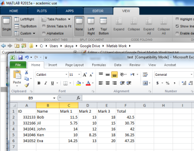
MATLAB have many builtin functions to work with Excel files. In this post, we will discuss some of the common functions to work with Excel files.  It is easy to interact with an excel file using xlswrite and xlsread commands. First we will make an sample excel file test.xlsx which contain grades of students in a class.

xlsread ( ) - Read Microsoft Excel spreadsheet file

The xlsread function reads data from the first worksheet of a Microsoft Excel file and save the numeric data in a array. If the file contains only numeric data the syntax is:
A = xlsread(‘filename’)
The ‘filename’ is a string with full name of the excel file (with path if the file is not in the current folder). The numeric data in the first work sheet of the file will be saved to the variable A. There are optional arguments to set the work sheet and the range to be read.
A= xlsread(‘filename’, ‘worksheet’, ‘range’)
The range is specified in the same way as represented in the excel equations (e.g. C2:F12).
If the file contains nonnumeric data, the syntax is modified as:
[NUM,TXT,RAW]=xlsread(‘filename’, ‘worksheet’, ‘range’)
The dat in the file will be saved as, numeric data in the variable NUM, text data in the variable TXT and the unprocessed data will be save as a cell array RAW. The cell array RAW will contain all the data in the worksheet.

Example:
Consider the file test.xlsx, which contain the grades of students. The numeric data is stored in the range C2:F6.
>> a=xlsread('test.xlsx', 'C2:F6')
a =
   11.5000   13.0000   18.0000   42.5000
    5.7500   10.0000   15.0000   30.7500
   14.0000   12.0000   16.0000   42.0000
   10.0000    8.2500   18.0000   36.2500
   14.2500   13.0000   20.0000   47.2500
To read all the data,
>> [a,b,c]=xlsread('test.xlsx')
a =
   1.0e+05 *
    3.3213       NaN    0.0001    0.0001    0.0002    0.0004
    3.3217       NaN    0.0001    0.0001    0.0001    0.0003
    3.4104       NaN    0.0001    0.0001    0.0002    0.0004
    3.4105       NaN    0.0001    0.0001    0.0002    0.0004
    3.4105       NaN    0.0001    0.0001    0.0002    0.0005

b =
    'ID'    'Name'    'Mark 1'    'Mark 2'    'Mark 3' 'Total'
    ''      'Bob'     ''          ''          ''          ''    
    ''      'Jil'     ''          ''          ''          ''    
    ''      'John'    ''          ''          ''          ''    
    ''      'Ken'     ''          ''          ''          ''    
    ''      'Eva'     ''          ''          ''          ''    

c =
'ID'       'Name'    'Mark 1'     'Mark 2'    'Mark 3' 'Total' 
[332133]    'Bob'     [11.5000]    [  13]    [  18]  [42.5000]
[332166]    'Jil'     [ 5.7500]    [  10]    [  15]  [30.7500]
[341041]    'John'    [     14]    [   12]   [  16]  [     42]
[341046]    'Ken'     [     10]   [8.2500]   [  18]  [36.2500]
[341052]    'Eva'     [14.2500]    [   13]   [  20]  [47.2500]

readtable( ) - Create table from file


readtable function is used to read not only excel files. \it read from different file types and sane as a MATLAB table.
T = readtable(‘filename’) is the basic syntax. There are optional arguments to set the file type and many other attributes based on the type of the file.
Example:

>> T = readtable('test.xlsx')

Warning: Variable names were modified to make them valid MATLAB identifiers.

T =

        ID         Name      Mark1    Mark2    Mark3    Total

    __________    _______    _____    _____    _____    _____

    3.3213e+05    'Bob'       11.5      13     18        42.5

    3.3217e+05    'Jil'       5.75      10     15       30.75

    3.4104e+05    'John'        14      12     16          42

    3.4105e+05    'Ken'         10    8.25     18       36.25

    3.4105e+05    'Eva'      14.25      13     20       47.25

      3.42e+05    'James'     12.5      13     20        45.5

      3.42e+05    'Anna'        12    10.5     16        38.5


Like in the xlsread function, read table also have optional arguments to read a specific worksheet and range. For more details refer Matlab Help.

Friday, July 15, 2016

Working with Text files in MATLAB - Part 2


In part one we discussed about basic functions to deal with text files. Now we will discuss more function to read from and write to different types of text files.

csvwrite( )  - Write comma-separated value file

csvwrite is the basic function in MATLAB to write data to a file as comma-separated values. It has only limited options to write numeric data to the file. The syntax is:
csvwrite(filename, C)
The function writes matrix C into the file as comma-separated values.

Example:
>> csvwrite('csvexample.txt',data)
Write the contents of the variable data to the file csvexample.txt as comma separated values.
If you want to write with more formatting options, you have to use fprinf or dlmwrite functions.

csvread( ) - Import Comma-Separated Data

Like csvwrite function, csvread also is simple function to read a .csv file or range of comma-separated numeric data and save to a matrix. The file must contain only numeric values.
X = csvread('filename')
Other optional arguments are offset and range.
X = csvread('filename', R, C, [range])
Where R and C are the row and column offsets and the range is row and column numbers of left top and right bottom points defined as range = [R1 C1 R2 C2].
Example:
To read the data from the csvexample.txt file we made in the previous example:
>> A=csvread('csvexample.txt')
A =
     1     2     3     4
     5     6     7     8
     9    10    11    12

dlmwrite( ) - Write matrix to ASCII-delimited file

dlmwrite function also is used to write the data in to a file. But it has more options than the csvwrite function. The syntax is:
dlmwrite('filename', C, 'delimiter', ’value’, R, C)
The function writes the contents of matrix C in to the file.  The delimiter is used to separate the values. The default delimiter is ‘,’ (comma). You can us other values also as the delimiter. The offset values R and C are optional.
There are optional user configurable attributes available to have more control over writing the data. ‘-append’ , ‘precision’, ‘newline’ are some commonly used attributes.
Example:
>> dlmwrite('dlmexample.txt',data)
Will write the contents of the variable data to the file dlmexample.txt as shown below
1,2,3,4
5,6,7,8
9,10,11,12
Now if we modify our command using different delimiter the file will be updated as:
>> dlmwrite('dlmexample.txt',data,'delimiter',';')
1;2;3;4
5;6;7;8
9;10;11;12
Note that the delimiter is changed to semi-colon.
>> dlmwrite('dlmexample.txt',data,'delimiter','\t')
1   2   3   4
5   6   7   8
9   10  11  12
Now the de limiter is the tab.
dlmwrite('dlmexample.txt',data,'delimiter','\t','precision','%.6f')
1.000000    2.000000    3.000000    4.000000
5.000000    6.000000    7.000000    8.000000
9.000000    10.000000   11.000000   12.000000
The ‘precision’ attribute is used to set the number of significant digits to 6.

dlmread( ) - Import Delimited Numeric Data

This function is used to read a file or a range of numeric data separated by any delimiter to a matrix. The file must contain numeric data only. The Syntax is:
X = dlmread(‘filename, ‘delimiter’, [range])
Delimiter and range are optional. If the delimiter argument is not specified, then the delimiter is inferred from the formatting of the file (consecutive white spaces are treated as a single delimiter). Range is to define the range of data to be read from a file, as explained in the csvread section.
Example:
>> A=dlmread('dlmexample.txt')
A =
     1     2     3     4
     5     6     7     8
     9    10    11    12
To read only 3rd row of the file:
>> A=dlmread('dlmexample.txt','\t', [2 0 2 3])
A =
     9    10    11    12

type( ) - Display contents of file

type is the function to display the contents of a file in the command window. The contents of the file may be numeric or non-numeric. The syntax is:
type ‘filename’

Example:
>> type 'dlmexample.txt'
1.000000  2.000000  3.000000  4.000000
5.000000  6.000000  7.000000  8.000000
9.000000  10.000000 11.000000 12.000000

>> type 'texttest.txt'
Welcome to Electrical Engineering Tutorial

>> type 'test.txt'
% This is a grade file
     jim 99 87 98
     jess 94 92 91

     jenna 100 90 95

Saturday, July 2, 2016

Working with Text files in MATLAB - Part 1


MATLAB can import text files both interactively and programmatically. Import Tool used to import data interactively. The Import Tool supports text files, including those with the extensions .txt, .dat, .csv, .asc, .tab, and .dlm. Data in these files can be a combination of numeric and nonnumeric text, and can be delimited by one or more characters.
There are many inbuilt functions to import and export data from and to the text files programmatically. Most of the import functions for text files require that each row of data has the same number of columns, and they allow to import a specified a range of data.
We will discuss some of the common functions to work with text files.

textread( ) - Read formatted data from text file

textread is a function which handles many of the problems/tasks of file input. textread is a function that "takes in" the name of a file and "returns" an array of information.
General syntax is
A = textread('filename', ' ', N, ’param’, value, ...)
X = textread('filename') reads numeric data from  the file into a single variable X.
Param and value are optional arguments to configure the output. One common parameter is ‘headerline’. It is used to tell textread to skip the first line of the file (the non-data line). Use the optional argument "'headerlines', number" where number is how many lines to skip.
X = textread('data', 'headerlines', 1);
There are many other types of parameters to configure the output. For the full list refer the Matlab help.
Suppose you wanted to read a file with strings in it as well as numbers. To do this, you must specify the "%format" of each column of data.
[A,B,C, ...] = textread('filename', 'format specifier', N, ’param’, value, ..) reads data from the file into the variables A,B,C,etc.  The type of each return argument is given by the format specifier string.  The number of return arguments must match the number of format specifiers in the FORMAT string.
N is another optimal argument to read a specific number of values to read from the file.  
A = textread('filename', '%d', 1); %  This reads a single integer from the file.

Example:

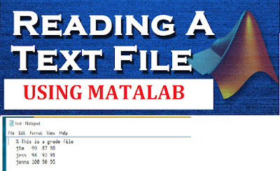
Consider the file test.txt, whose content is:
            % This is a grade file
            jim 99 87 98
            jess 94 92 91
            jenna 100 90 95
     
To read this file we use:
>> [names, grade1, grade2, grade3] = textread('test.txt', '%s %f %f %f', 'headerlines', 1)
names =
    'jim'
    'jess'
    'jenna'
grade1 =
    99
    94
   100
grade2 =
    87
    92
    90
grade3 =
    98
    91
    95
To read all numeric data from a delimited text file, use a single output argument, empty format string, and use the appropriate delimiter.
Example:
Suppose delimexample.txt contains:
        1,2,3,4
        5,6,7,8
        9,10,11,12

To read the whole matrix into a single variable:
>> [data] = textread('delimexample.txt','','delimiter',',')
data =
     1     2     3     4
     5     6     7     8
     9    10    11    12    

textscan( ) – Read Formatted Data from a Nonrectangular Text File

The textscan function is used to read formatted text file and save data to a cell array. The synatax is similar to the textread function. Here to read multiple data we don’t need to specify the multiple output variables, but the whole data will be stored as a cell array. The syntax is:
C = textscan(FID, 'format specifier')
Other optional arguments are very similar to the textread function.
When textscan reads a specified file or string, it attempts to match the data to the format string. If textscan fails to convert a data field, it stops reading and returns all fields read before the failure.
Example:
Consider the test.txt file in the previous section. To read the file content to a cell array C:
>> fid = fopen ('test.txt', 'r+');
>> C = textscan(fid, '%s %f %f %f', 'headerlines', 1);
>> celldisp(C)
C{1}{1} =
jim
 C{1}{2} =
jess
 C{1}{3} =
 jenna
 C{2} =
    99
    94
   100
C{3} =
    87
    92
    90
C{4} =
    98
    91
    95

The textscan function can be used to read data in a string. The syntax is:
C = textscan(string)